Messing with probabilities (part 1: The math)

[Edit: This is no longer "part 1", but the whole article. See "How I screwed myself over with side effects".]

In the mini-project I was thinking of recently there are a lot of coin flips. They usually occur in groups of one to eight, and I only want to know the total amount of heads. Now, I could simply flip that digital coins that many times and be done with it, or I could be a bored college student who actually should be doing other things right now, and think of something more sophisticated.

For something so trivial, there must be a way to reduce the several random flips to ONE random number generation. It's just a matter of dividing the [0, 1]-space into the right intervals, to maintain the same probability for every outcome.

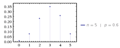
Having cursory knowledge of statistics, my thoughts immediately wandered to something called the binomial distribution. In short, a binomial distribution with parameters n and p - denoted as B(n, p) - describes the chance that x out of n trials with chance p to succeed, will succeed. For example, here is the probability distribution function f(x) (or, in this case, probability mass function, since it's discrete) for B(5, 60%).

This chart tells us that the chance that if we try something that has a 60% chance to succed five times, our chance to succeed twice is around 25%.

It's not hard to notice that getting heads on a coin flip is a random trial with a chance to succeed of 50%. Thus, B(n, 50%), where N is the amount of coins flipped, perfectly describes what I'm trying to achieve!

Calculating the PDF for B(n, p) is a fairly trivial matter, just translating a formula. Here's the Clojure:

(defn binomial [n k]
  (letfn [(fact [n] (reduce * 1 (range 2 (inc n))))]
    (/ (fact n) (fact (- n k)) (fact k))))

(defn binom-pdf [n p]
   (fn [x]
    (if (<= 0 x n)
      (* (Math/pow (- 1 p) (- n x)) (Math/pow p x) (binomial n x))
      0)))

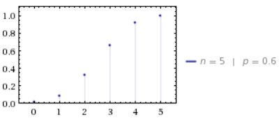
So, now we have the PDF for B(n, p). There's another, related function, called the cumulative distribution function. It's a function F(x) that describes the chance that the result will be less than x. Seems like a weird thing to devote an entire function to, but it's surprisingly useful in practice. The CDF for B(5, 60%) looks like this:

And, the PDF again:

The CDF is simply the sum of all the PDF entries for values less than x. For example, in this case, CDF(3) = PDF(0) + PDF(1) + PDF(2) + PDF(3). This is why the CDF is always rising, and why the final value is exactly equal 1 (= 100%).

Using the cumulative distribution function, we can now map one single random number to a final result. Just for reference, the values of this CDF are roughly:
CDF(0) = 0.01
CDF(1) = 0.087
CDF(2) = 0.317
CDF(3) = 0.663
CDF(4) = 0.922
CDF(5) = 1

Thus, we have a set of intervals, that each corresponds to a result:

[0, 0.01) => 0
[0.01, 0.087) => 1
[0.087, 0.317) => 2
[0.317, 0.663) => 3
[0.663, 0.922) => 4
[0.922, 1] => 5

Which solves the original problem: We divided [0, 1] into intervals that maintain the same weight for every possible outcome. Now, we can just generate one random number, pick the interval it belongs to, and we have our final result.

And how to more-or-less elegantly do that in code, I'll show in the next post (actually, the post AFTER the next one - there's another thing I want to interject first).